
Six Sigma tools and trading might seem worlds apart — one focuses on improving processes, the other on profiting from market moves. But at their core, both rely on statistics to measure performance, understand variability, and predict outcomes. Let’s explore how the two connect.
1. Standard Deviation — Measuring Spread
1.1 Connecting Six Sigma Tools and Trading
In Six Sigma:
Standard deviation (σ) measures how far individual results deviate from the mean. A lower σ means more consistent results.
In Trading:
Standard deviation measures price movement from an average over time. Tools like Bollinger Bands use it to define expected ranges.
- Low σ → Stable prices
- High σ → Large price swings
The Link:
In both, σ tells you how consistent (or volatile) something is — in quality control, less variability is better; in markets, variability is both risk and opportunity.
2. The Bell Curve — Understanding Probability
In Six Sigma:
The bell curve (normal distribution) shows the likelihood of outcomes:
- ~68% within ±1σ
- ~95% within ±2σ
- ~99.7% within ±3σ
In Trading:
A bell curve can model daily price changes — though real markets often have “fat tails” (more extreme events than a perfect curve predicts).
- ±1σ → Normal price moves
- ±2σ or ±3σ → Rare events, often news-driven
The Link:
Both use the curve to understand probability — Six Sigma to control defects, traders to gauge unusual moves.
3. Variance — The Foundation for Risk
In Six Sigma:
Variance measures how far data spreads from the mean, squared. High variance means large fluctuations.
In Trading:
Variance underpins risk metrics like Sharpe Ratio and Value at Risk (VaR). Higher variance means higher uncertainty — and potentially larger losses or gains.
The Link:
Variance is a universal measure of stability vs instability.
4. Volatility — Trading’s “Process Variability”
In Six Sigma:
Volatility isn’t a formal term, but “process variability” is — and the goal is to reduce it.
In Trading:
Volatility measures how much and how quickly prices move. It’s calculated using standard deviation or other measures like ATR (Average True Range).
The Link:
Trading volatility is just process variability applied to markets. High volatility = unpredictable process.
5. Live Bell Curve in Action — Using Multi-Level Bollinger Bands
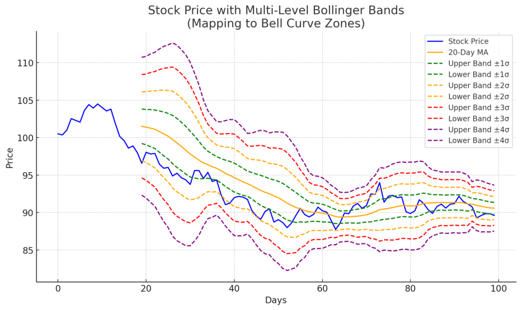
When you extend Bollinger Bands beyond the standard ±2σ to include ±1σ, ±3σ, and ±4σ, you essentially map the bell curve onto price action in real time.
| Band Level | Bell Curve Equivalent | Probability Zone | Trading Meaning |
|---|---|---|---|
| ±1σ | First hump edges | ~68% of prices | Normal daily volatility |
| ±2σ | Wider curve section | ~95% of prices | Breakouts become notable |
| ±3σ | Far edges | ~99.7% of prices | Rare moves, possible reversals |
| ±4σ | Extreme tail | <0.01% | Black swan-level events |
Why it’s “Live”:
- The mean is your moving average.
- The σ values are recalculated daily.
- Bands expand in volatile markets (flatter bell curve) and contract in calm markets (narrower bell curve).
Trading Use:
- Mean Reversion: Price beyond ±2σ or ±3σ has a higher chance of snapping back.
- Breakout Signals: Sustained moves outside ±2σ may start strong trends.
- Volatility Gauge: The width of the curve shows market energy at a glance.
Bottom Line:
Six Sigma and trading both live in the world of measuring, analyzing, and controlling variability. In manufacturing, that means fewer defects; in markets, it means reading probabilities in real time — and sometimes, using tools like multi-level Bollinger Bands to literally watch a bell curve move across your chart.
Originally posted 2025-08-13 02:23:43.
